After a technical measure on a wind turbine, the question often arises as to what change the measure will have on the performance of the system. For example, you would like to know how much additional performance the calibration of a nacelle misalignment brings.
First of all, it is close to the performance curve of the system in the periods before and
to be compared with each other after the measure. In this article, we highlight the inaccuracies of this approach and present a more precise approach through which reliable performance curve comparisons can be made using machine learning.
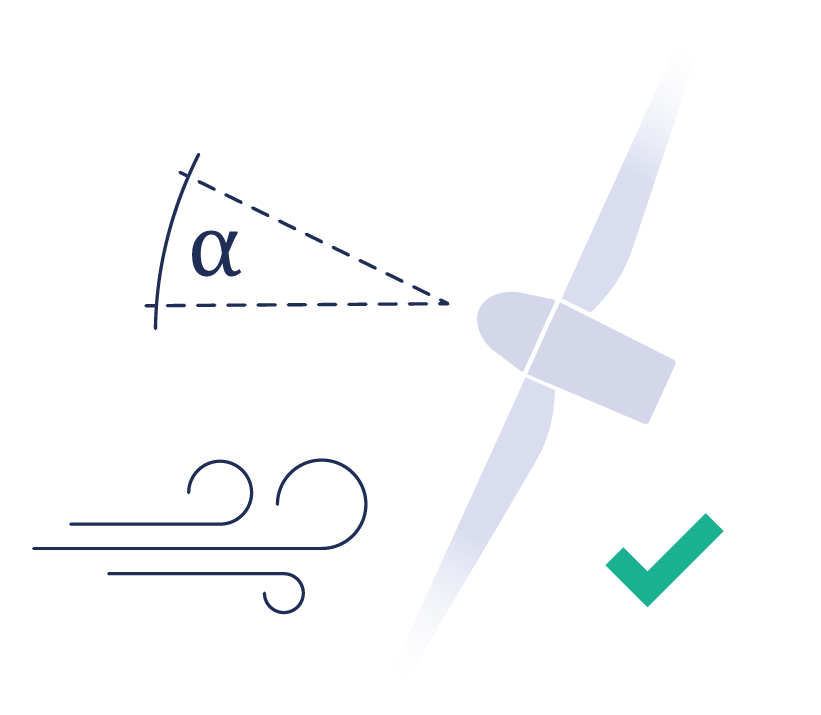
Optimization of the Yaw Error
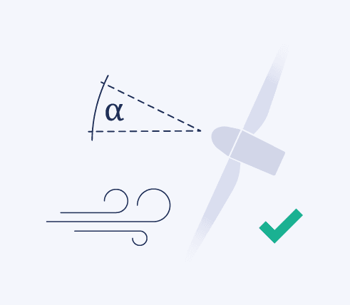
When correcting a nacelle misalignment, it can be assumed that the calibration of a systematic nacelle misalignment leads to an improvement in the performance of a wind turbine. We have this in detail in described in this article.
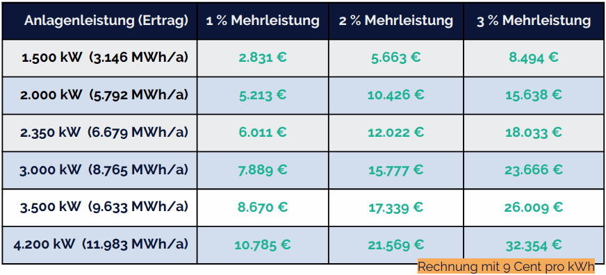
Theoretical additional returns
If you add up the annual yields of a wind turbine with a theoretical additional output of 1-3%, you can quickly see the benefit of a nacelle misalignment calibration.
Proof of increased yield

The question, however, is how this increase in performance can be demonstrated.
The process of converting kinetic wind energy into electrical energy is
very complex and highly dependent on
meteorological parameters.
The problems of a simple performance curve comparison
If you make a change to a wind turbine, you want to know how much this change changes the performance of the system. However, the performance of a wind turbine does not only depend on the wind speed. This means that the performance curve (power per wind speed) changes under different meteorological conditions.In order to be able to identify exactly what cause, for example, a calibration of the wind direction tracking has on the power curve, a normal power curve comparison of two periods is not sufficient, as the meteorological conditions can also change over periods of years.
Dependence of the performance curve on the air density
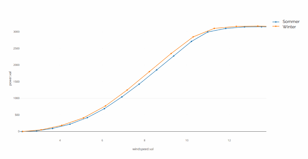
Apart from wind speed, air density is one of the most important factors affecting the performance curve of wind turbines. At the same wind speed, the energy content of the wind changes depending on the air density. The denser the air, the more energy the wind has and the more power the wind turbine can convert from the wind.
Air density depends mainly on temperature, air pressure and humidity.
In the figure on the left you can see a clear difference in the performance curve of a system between summer and winter.
Dependence of the power curve on the turbulence intensity
Similarly, the power at the same wind speed depends on the turbulence intensity
We cannot therefore assume that the power curve of two time-separated measurements is comparable if we only measure the wind speed.
Validated approach: Machine Learning
Neural networks are very good at learning complex relationships. The non-linear and therefore complex relationship between the meteorological parameters and the performance of a wind turbine can be learned very well from historical SCADA data using this method. The 10 minutes of data are used as input data for the model and used to train the model, which predicts the performance of the test system.
Before calibration
The neural network learns the complex performance behavior from different wind directions, air pressures and wind speeds. Applying this model to new data allows you to simulate the performance of the test facility for different weather conditions.
After calibration
If you now calibrate the nacelle misalignment of the test system, for example, then the simulation can be compared with the real measured data. The determined performance difference, which is adjusted for the location and meteorological conditions, can be used to evaluate the success of the measure.
1. Training
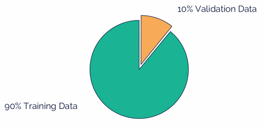
We only use part of the data (training data) to train the performance curve. This gives us a data set (validation data) with which we can check how well the neural network's performance prediction works.
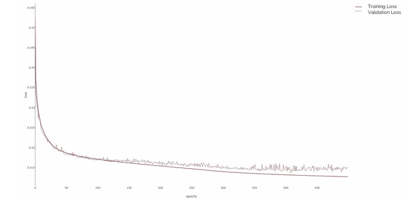
2. Training Loss vs Validation Loss
If we now compare the error of our training from the training data and from the validation data, we must ensure that so-called over fitting does not occur, i.e. the neural network learns the training data by heart, but only understands the basic connections.
3. Self Consistency Check

To see whether the network has learned the performance behavior well, we use historical data from the complete training and validation data set and check how well the simulation works.
In most cases we achieve 99% accuracy.
4. Performance comparison
Finally, we use data as input that was measured during the test period, e.g. after calibration, and compare the results of the machine learning model with the actually measured values. The difference then results in the increased performance or reduced performance.

If you integrate these differences over a certain period of time, you get a direct difference in kWh between the expected and actually generated power of the test system
